
· By Sajeevan (Saj) Veeriah
Machine vision · 5 min read
Before training the model, do the camera maths
A worked example of field of view, exposure and motion blur, and how to tell whether an inspection image contains enough evidence.
A camera looks down at a moving part. The inspection model reports a defect with confidence. On the next batch, apparently similar defects are missed. Before changing the network or collecting thousands more labels, there is a cheaper question to answer: what evidence actually reached the sensor?
Consider a fictional conveyor inspecting a 0.2 mm surface feature at 1 m/s. The requirement sounds like a machine-learning problem. It is also an optics, lighting and timing problem. A few calculations help separate those parts before they become an expensive dataset.
Give the feature a pixel budget
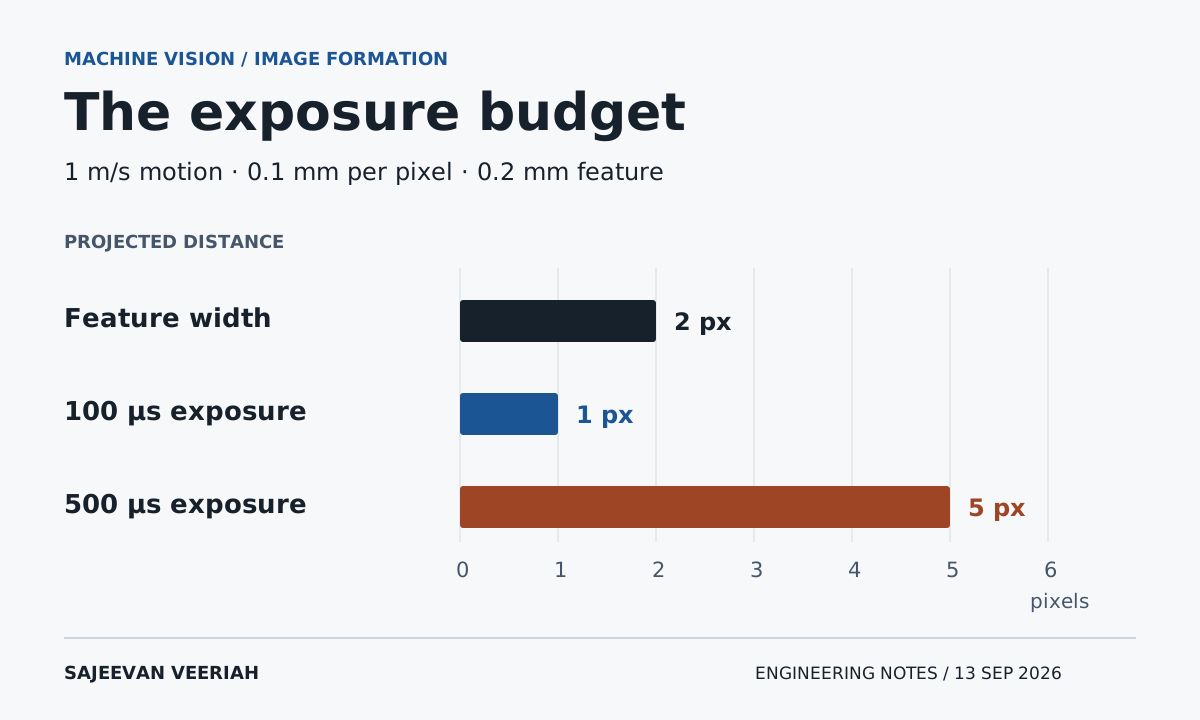
Suppose the camera sees 200 mm across the direction of travel, sampled by 2000 pixels. At the inspection plane, the nominal scale is 200 / 2000 = 0.1 mm per pixel. A 0.2 mm feature therefore spans just two pixels along that axis.
That ratio describes geometric sampling. It does not establish that the feature can be detected, measured or classified reliably. Focus, lens contrast, noise, feature orientation and the position of an edge relative to the pixel grid still matter. Two samples across a feature leave little room to distinguish its shape.
Write down the required decision first. Detecting a dark mark is different from measuring its width or deciding whether it is a crack. Set the required image scale through trials on representative parts and known features. Avoid treating a camera megapixel count as a complete inspection specification.
The part keeps moving while the shutter is open
For uniform motion parallel to the image plane, projected travel in pixels is speed × exposure time / object-space millimetres per pixel. The quantities must use consistent units. At 1 m/s, the part moves at 1000 mm/s.
With a 500 µs exposure, it travels 1000 × 0.0005 = 0.5 mm, or five pixels at our chosen scale. The original feature was only two pixels wide. This does not calculate a detection probability; it shows that motion can spread its image across a distance larger than the feature itself.
At 100 µs, the travel is 0.1 mm, or one pixel. Basler recommends, as a general rule for moving objects, keeping movement during exposure to no more than one pixel. That is a useful starting constraint, not an acceptance test for every inspection.
| Exposure | Calculated travel at 1 m/s |
|---|---|
| 500 µs | 0.5 mm = 5 pixels |
| 100 µs | 0.1 mm = 1 pixel |
| 50 µs | 0.05 mm = 0.5 pixels |
Sources: [1]
Shorter exposure creates a lighting decision
Reducing exposure from 500 µs to 100 µs cuts the collection time to one fifth. With unchanged illumination and a linear, unsaturated response, the sensor collects approximately one fifth as many signal photons. Maintaining a similar photon count would require approximately five times the irradiance at the sensor, or another change to the optical arrangement.
That is an idealised exposure comparison, not a recommendation to turn a lamp up fivefold. The part may be reflective, the light may have thermal or pulse limits, and the lens aperture also affects focus tolerance. Confirm the actual lighting and camera limits.
Increasing gain makes the output brighter, but Basler notes that it amplifies signal and noise. It does not replace missing optical evidence. A useful lighting trial changes the angle and diffusion as well as intensity, then checks whether the feature remains distinguishable across the expected surface finishes.
Sources: [1]
Frame rate and exposure answer different questions
A camera delivering 100 frames per second has a nominal 10 ms interval between frames. That number does not say whether each frame was exposed for 50 µs or 5 ms. The first controls sampling cadence; the second controls the duration over which motion is integrated.
Record the effective exposure and trigger behaviour for the selected camera, rather than assuming a requested setting is the complete timing contract. Basler documents model-dependent exposure ranges and cases where effective exposure differs from the set value. No camera model is being selected in this example.
For a triggered conveyor inspection, also check that the intended part is inside the useful field of view when exposure occurs. A sharp picture of the wrong location is still an unusable inspection.
Sources: [2]
Run a capture experiment before a training experiment
Use representative acceptable and defective test parts with an independently established reference. Capture them stationary first, then at the intended speeds. Keep the original images and acquisition settings, including any automatic settings, so a later comparison remains meaningful.
| Comparison | Question it answers |
|---|---|
| Stationary versus moving, same settings | Does motion remove useful detail? |
| Exposure sweep, lighting recorded | Can the motion limit be met with usable contrast? |
| Expected part heights and surface finishes | Does the optical setup tolerate normal variation? |
| Repeated passes and separate acquisition sessions | Does performance survive more than one convenient capture? |
When evaluating a model, keep repeated images of the same physical part together when separating training and test data. Also reserve genuinely separate parts or acquisition sessions appropriate to the deployment question. Otherwise, near-duplicate images can make the evaluation easier than the real task.
Measure missed defects and false rejects against the reference, with their sample counts. Inspect failures alongside the original images. A confidence score alone cannot tell you whether the camera supplied the evidence needed to make the decision.
The useful handover is a capture specification: required field of view, acceptable focus range, exposure and lighting conditions, timing behaviour, and measured inspection performance within those conditions. That gives the model a defined physical problem to solve.
Sources and further reading
Sources checked on 13 September 2026. Conveyor dimensions, speeds and test cases are illustrative. Calculations assume uniform projected motion and a constant image scale at the inspection plane; they are not camera qualification or production results.