
· By Sajeevan (Saj) Veeriah
Sensing and signal processing · 4 min read
A smooth sensor trace can hide real motion
How an 80 Hz signal becomes indistinguishable from 20 Hz when sampled at 100 samples per second, and what to check before trusting a trend.
A trend can look calm while the machine is doing something much faster. The display may be drawing every value it received correctly. The missing information can have disappeared before those values reached the screen.
Consider a fictional vibration measurement containing an 80 Hz component. A logger stores 100 samples per second. That sounds like a busy stream of data, but the numbers alone cannot distinguish this signal from a much slower one.
Two motions, one set of numbers
Take a unit-amplitude cosine: x(t) = cos(2π × 80 × t), with time in seconds. At 100 samples per second, the sample times are t = n / 100 for integer n.
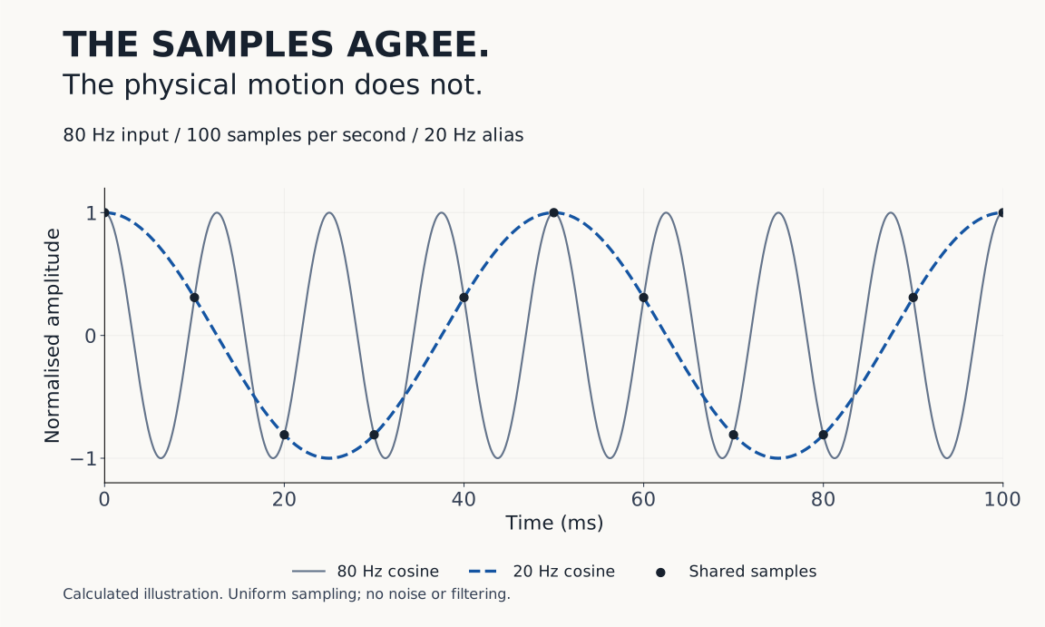
The sampled values are cos(1.6πn). For integer n, these equal cos(2πn - 0.4πn), which equals cos(0.4πn). That is exactly the sequence produced by a 20 Hz cosine sampled at the same times. The chart shows both continuous curves and their shared sample points.
At 0, 10, 20, 30 and 40 ms, either signal produces approximately 1.000, 0.309, -0.809, -0.809 and 0.309. A smoother line between these dots cannot tell us which physical signal created them. This ambiguity is aliasing.
| Quantity | Value in this example |
|---|---|
| Actual cosine frequency | 80 Hz |
| Sampling interval | 10 ms |
| Sampling rate | 100 samples/s |
| Indistinguishable lower frequency | 20 Hz |
Specify the bandwidth before the rate
For ordinary baseband acquisition of a band-limited signal, sample above twice its highest frequency. A practical design also needs room for the anti-alias filter's transition band. Analog Devices' MT-002 explains why unwanted input frequencies must be attenuated before sampling.
That requirement concerns everything that can reach the sampler, including interference. A process variable may change slowly while electrical noise or mechanical vibration adds faster components. Filtering after those components have folded into the useful band cannot uniquely recover the lost distinction.
Sources: [1]
Follow the value through every rate change
For a proposed measurement chain, I would write a rate beside each stage: sensor conversion, internal filtering, bus delivery, application processing, stored records and screen updates. Then I would identify what happens when a stage discards values.
A hypothetical sensor could convert at 1000 samples/s while an application stores one value in every ten. That creates a new 100 samples/s sequence. An 80 Hz component must be removed before that reduction if the stored data is intended to represent only frequencies below 50 Hz.
Filtering and decimation are deliberate parts of converter design. Analog Devices' discussion of sigma-delta conversion describes digital filtering before lowering the output rate. Reading a register more often does not establish that it contains a new conversion.
| Stage to inspect | Evidence to retain |
|---|---|
| Sensor output | Configured rate, filter mode and data-ready behaviour |
| Transport | Sequence numbers, dropped values and acquisition timestamps |
| Stored series | Resampling rule and filtering before reduction |
| Display | Whether points are selected, averaged or summarised |
Sources: [2]
Make the measurement disagree with itself
A useful bench experiment starts with a known input, within the equipment's limits, and an independent reference. Sweep the input frequency while keeping amplitude and acquisition settings recorded. Compare the stored result with the reference, including frequencies outside the intended measurement band.
Repeat selected points with a different sample rate. In our ideal example, changing from 100 to 120 samples/s moves the 80 Hz component's lower-frequency alias from 20 to 40 Hz. That movement is a diagnostic clue, not proof that every changing peak is an alias.
The chart assumes uniform sampling, exact frequencies and no noise. Real tests must also inspect timing variation, clipping, filter response and sample loss. Keep raw acquisition timestamps wherever available so these effects can be separated.
The acceptance criterion should describe what the measurement must preserve: a defined frequency band, tolerable amplitude and timing error, and adequate rejection outside that band. A visually smooth trace is not an acceptance criterion.
Sources: [1]
Sources and further reading
References checked on 16 September 2026. The second reference is historical technical material with no publication date established here. Frequencies and curves are an original illustrative calculation, not a hardware test or product recommendation.